What Is A Perceptron?

What Is A Perceptron?

What Are We Trying to Model?

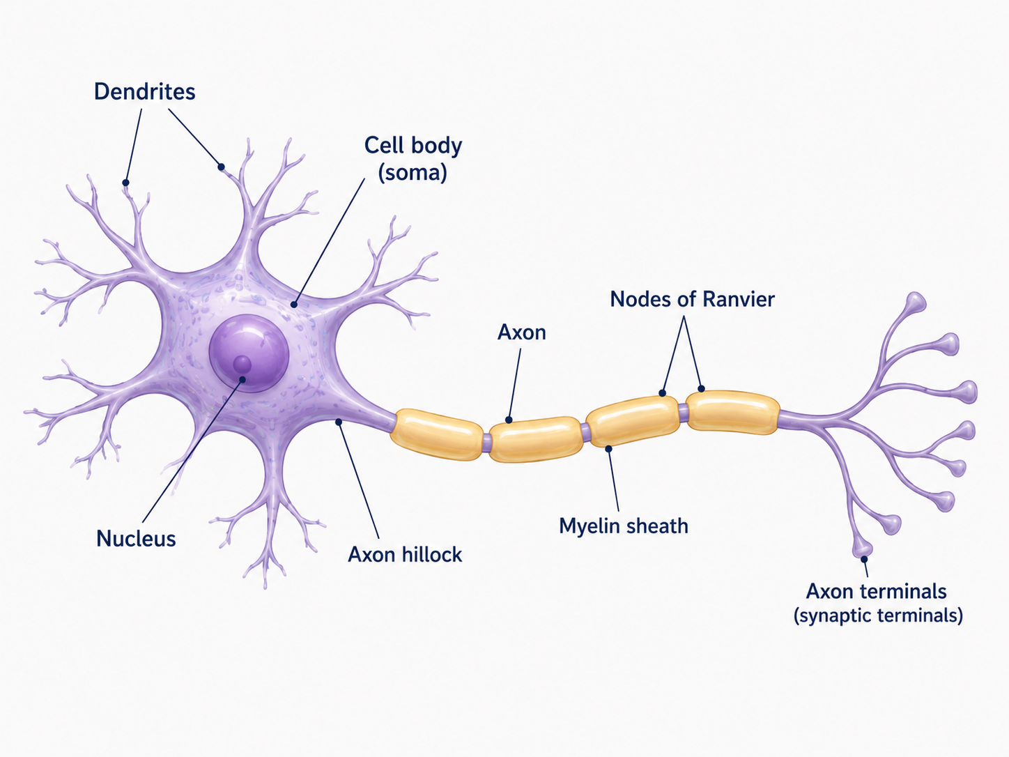
Let’s first begin with what a perceptron is trying to model. A perceptron is a simplified version of a brain cell. These biological neurons are interconnected with potentially thousands of other neuron. One end, where the dendrites are, recieves the electrical and chemical signals from other neurons. Then if the signals recieved trigger the neruon to fire, the signal moves down the axon to the other end of the neruon where the axon terminals are which connect to many other nerons. Now, I do want to say that there is a lot more that can be explained here when it comes to brain cells and how they work and what we still don’t know and since I am not a neuroscientist I don’t know any of it. But, this all we need to know to move on so let’s continue.

An illustration of a single brain cell.

The Beginnings Of The Artifical Neuron

Warren McCulloch and Walter Pitts were the first to publish the concept of a simplified neuron 1943 in their paper title “A Logical Calculus of the Ideas Immanent in Nervous Activity” in the Bulletin of Mathematical Biophysics. This is the so-called McCulloch-Pitts (MCP) neuron. They described the biological neuron as a simple logic gate with binary outputs. Multiple signals arrive at the dendrites, they are the integrated into the cell body, and, if the accumulated signal reaches a certain threshold, an output signal is generated which moves down the axon to the axon terminals.

A couple of years after Warren McCulloch and Walter Pitts published their paper, Frank Rosenblatt published the first concept of the learning rule based on the MCP neuron model. His paper was titled “The Perceptron: A Perceiving and Recognizing Automaton” which was published in 1957. He proposed a an algorithm that automatically learn the optimal weight coefficients for the input features. This sum of the product of the features with the weight coefficients would then be used to determine whether or not the neuron fires or not. The example we will be using later is the supervised learning task of classification. So in this context the perceptron can be used to classify an example as either belonging to the class of interest or not.

The Mathematics Of A Peceptron

In the context of binary classification, we can refer to our two classes as either 1 (positive class) or -1 (negative class). We then define a decision function \(\phi(z)\) that takes in a linear combination of the weight coefficients and the features. \(z\) is called the net input. We will use \(\textbf{w}\) for the weight vector and \(\textbf{x}\) for the input vector. Therefore we would have the following:

\[ \mathbf{w} = \begin{bmatrix} w_1 \\ \vdots \\ w_m \end{bmatrix}, \qquad \mathbf{x} = \begin{bmatrix} x_1 \\ \vdots \\ x_m \end{bmatrix} \]

and

\[ \begin{align*} z &= \textbf{w}^T \textbf{x}\\ &= w_1x_1 + w_2x_2 + \cdots + w_mx_m \end{align*} \]

If the the net input of a particular example is greater than a predefined threshold, say \(\theta\), then we predict 1 or -1 otherwise. In the perceptron algorithm the decision function is defined as the following:

\[ \phi(z) = \begin{cases} 1, & \text{if } z \geq \theta, \\ -1, & \text{otherwise.} \end{cases} \]

We can simplify this function by moving \(\theta\) to the left side of the equation and defining a weight \(w_0 = -\theta\) and \(x_0 = 1\). Then \(z\) can be written as:

\[ \begin{align*} z &= \textbf{w}^T \textbf{x}\\ &= w_0x_0 + w_1x_1 + w_2x_2 + \cdots + w_mx_m \end{align*} \]

The weight \(w_0 = -\theta\) is called the bias unit.

The Perceptron Learning Algorithm

The overall algorithm for the perceptron is simple.

1. Initialize the weights to random small numbers.
2. For each training example:
   1. Compute the predicted value \(\hat{y}\).
   2. Update the weights.

The update for a particular weight, say \(w_j\), can be formally written as:

\[w_j := w_j + \Delta w_j\]

This means that we update \(w_j\) by adding to it a change in \(w_j\). \(\Delta w_j\) is defined to be the following:

\[\Delta w_j = \eta(y^{(i)} - \hat{y}^{(i)})x^i_j\]

To those who might have an adverse reaction to seeing a lot of mathematical symbols at once, fear not, this is simple to understand. \(\eta\) (eta) is called the learning rate and is usually a constant between 0.0 and 1.0. \(y^{(i)}\) is the true class label for the \(i\)th training example and \(\hat{y}^{(i)}\) is the predicted class label for the \(i\)th training example. Finally, we multiply by \(x^i_j\), which is the \(j\)th value for the \(i\)th training example.

Perceptron Code Example

Now we will look at an example of a perceptron written in python. The following code is not mine but taken from the book titled Python Machine Learning and can be found here.

import numpy as np

class Perceptron(object):
    """
    Perceptron classifier.
    
    Parameters
    ----------
    eta : float
        Learning rate (between 0.0 and 1.0)
    n_iter : int
        Passes over the training dataset.
    random_state : int
        Random number generator seed for random weight initialization.
    
    Attributes
    ----------
    w_ : 1d-array
        Weights after fitting.
    errors_ : List
        Number of misclassifications (updates) in each epoch.
    """

    def __init__(self, eta = 0.01, n_iter = 50, random_state = 1):
        self.eta = eta
        self.n_iter = n_iter
        self.random_state = random_state

    def fit(self, X, y):
        """
        Fit training data.

        Parameters
        ----------
        X : {array-like}, shape = [n_examples, n_features]
            Training vectors, where n_examples is the number of 
            examples and n_features is the number of features.
        y : array-like, shape = [n_examples]
            Target values.
        
        Returns
        ---------
        self : object
        """

        rgen = np.random.RandomState(self.random_state)
        self.w_ = rgen.normal(loc=0.0, scale=0.01, size=1 + X.shape[1])

        self.errors_ = []

        for _ in range(self.n_iter):
            errors = 0
            for xi, target in zip(X,y):
                update = self.eta * (target - self.predict(xi))
                self.w_[1:] += update * xi
                self.w_[0] += update
                errors += int(update != 0.0)
            self.errors_.append(errors)
        return self
    
    def net_input(self, X):
        """Calculate net input."""
        return np.dot(X, self.w_[1:]) + self.w_[0]
    
    def predict(self, X):
        """Return class label after unit step."""
        return np.where(self.net_input(X) >= 0.0, 1, -1)

I will first describe the three attributes of this class that are intitialized when the class is created. First, eta is the learning rate as mentioned before. n_iter is the number of times the algorithm will iterate through the entire training data. Lastly, random_state is the seed for the random number generator that will be used to initialize the model weights to random numbers.

Now, let’s move into the main function, the fit function. This function utilizes two other functions, the net_input and predict functions. I’ll explain those as we encounter them. The fit function first initializes the weights to random numbers using a standerd normal distribution in the following two lines.

rgen = np.random.RandomState(self.random_state)
self.w_ = rgen.normal(loc=0.0, scale=0.01, size=1 + X.shape[1])

Then we keep track of the errors for each iteration using the list self.errors_.

Now for the main part of the function, the for loop. The outer loop will iterate n_iter times and for each of those loops we will loop over all of the training data in the inner loop. The errors variable in the outer loop will keep track of how many errors were made after each time the inner loop has run. The number of errors will be appended to the self.errors_ list. In the inner loop we iterate through each training example using the following line of code, for xi, target in zip(X,y):. This use zip here so the we get a tuple where the first element is an array that contains the \(i\)th trainging example along with \(i\)th true class value. The tuple gets unpacked and put in the xi and target variables. We then compute part of the update using the following line.

update = self.eta * (target - self.predict(xi))

This line of code maps to the following mathematical expression, \(\eta(y^{(i)} - \hat{y}^{(i)})\).

We see that a predict function is used in the code here so let’s go into that next. The predict function is very simple, it either returns a 1 or a -1 as the prediction depending on whether the net_input function returns a value greater than or equal to 0 or not. The net_input function is simply the dot product of array xi and the weights self.w_. This returns a scalar. After we have the new update we add that to the current weights and the bias unit with the following code.

self.w_[1:] += update * xi
self.w_[0] += update

After that we get the errors made with errors += int(update != 0.0).

I do want to quickly mention that this class assumes that assumes that the array of true class labels, y, only contains 1’s and -1’s for it’s entries.

As this is my first blog post ever, I hope I did an okay job in explaining what a perceptron is and how it works. I hope this helps anyone looking for help in understanding what a perceptron is.